Comment lire la courbe temps-intensité d'un disjoncteur à coupure magnétique (MCCB)
Publié le : Auteur : Rachel
An MCCB datasheet curve is one of the few documents in electrical design that rewards five minutes of careful reading with months of avoided argument. It tells you, for any fault current, how long the breaker will take to open. It also tells you whether two breakers in series will trip in the right order — which is the part most specifications get wrong.
The problem is that the curve is printed on a log-log grid, in a corner of a PDF, with three settings overlaid and a shaded tolerance band that nobody explains. Reading it incorrectly is easy, and the errors are not obvious: a curve that looks selective at a glance can overlap over exactly the fault range that matters.
This is a reading guide, not a catalogue. It covers what the axes mean, where the three regions sit, how to read a specific fault current off a curve, and how to compare two curves so that the conclusion holds at the fault level your panel actually sees.
What an MCCB Time-Current Curve Actually Plots
The horizontal axis is prospective current — the current that would flow if the breaker were replaced by a solid link. The vertical axis is operating time — how long the breaker takes to open at that current. Both axes are logarithmic, because the useful range covers four decades of current and six of time.
Three things follow from that definition, and each is a common source of confusion:
The curve describes the breaker alone. It says nothing about the cable, the load, or the upstream device. Those are separate curves drawn on the same axes for comparison.
The current axis is usually in multiples of the setting, not in amperes. That makes one curve usable across a range of ratings, and it means you must convert your fault current into a multiple before reading.
The curve is a band, not a line. Manufacturing tolerance means the real trip time falls somewhere inside a shaded envelope. Reading the centre line and ignoring the band is how optimistic selectivity claims are made.
Reading the Two Log Axes
On a log axis, equal distances represent equal ratios, not equal amounts. The gap between 10 s and 100 s is the same width as the gap between 100 s and 1,000 s. Two practical consequences:
Axis
Typical span
How to read a point
Current (x)
About 0.5 to 20 times the setting, sometimes wider
Find the decade, then count the minor divisions — they are 2, 3, 4 … 9 within that decade, not equal steps
Time (y)
0.001 s to 10,000 s
Same rule: minor lines inside a decade are unevenly spaced, crowding toward the next decade
A reading taken by eye on a log grid is only good to about one minor division. That is why coordination studies use the published numerical data points rather than a screenshot of the curve, and why a selectivity conclusion should be checked against the manufacturer’s verified tables whenever one exists.
The Three Regions of the Curve
Every MCCB curve is built from the same three pieces, whatever the trip technology:
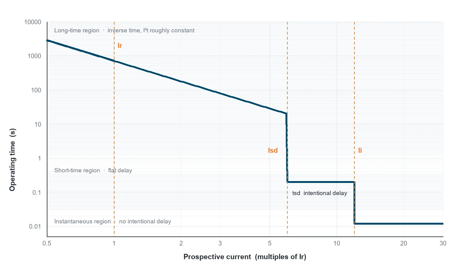
Long-time region. The overload zone, from about 1.05 times the setting upward. The curve falls steeply: doubling the current roughly quarters the time, because the thermal element responds to I²t. This is the region that protects the cable.
Short-time region. A deliberate flat section where the trip time is held constant while current rises. This exists only where the device has an intentional delay — an electronic trip unit, or a category B breaker. On a thermal-magnetic category A device this region is absent and the curve drops straight to instantaneous.
Instantaneous region. Below a set current multiple the breaker opens with no intentional delay, typically within one or two cycles. On the graph this is the near-vertical drop to the bottom of the time axis.
Reading a curve is mostly a matter of locating which region your fault current lands in. A 1.3 times overload is a long-time question; a 30 kA fault is an instantaneous question; the interesting design work happens where the two meet.
Knee Points: Ir, Isd, Ii and tsd
The transitions between regions are marked by the settings, and they are what you actually read off the curve.
Schematic curve shape, drawn to illustrate the axes and the knee points. It is not a manufacturer’s published curve — always read the curve for the specific device you are specifying.
Point
Where it sits
What it means when you read it
Ir
Start of the long-time region, at 1.0 on the current axis if the axis is in multiples of Ir
Below roughly 1.05 Ir the breaker does not trip at all; the curve begins just above it
tr
Time value of the long-time curve at 6 Ir
A single number summarising the whole thermal curve, because the shape is fixed once tr is set
Isd
Left edge of the flat short-time section
Fault currents above Isd are held for tsd instead of tripping immediately
tsd
Height of the flat section
The intentional delay. This is the number you grade between upstream and downstream devices
Ii
Right edge of the flat section, where the curve drops
Above Ii the breaker ignores tsd and trips instantaneously — the usual cause of a failed selectivity claim
A Worked Reading
Take a 250 A frame with an electronic trip unit set as follows: Ir = 0.8 (200 A), tr corresponding to the standard curve, Isd = 4 × Ir (800 A), tsd = 0.1 s, Ii = 10 × In (2,500 A). Read the curve at three fault levels:
Prospective current
Multiple de l'Ir
Region
Rough operating time
300 A
1.5
Long-time
Hundreds of seconds — the cable is allowed to carry a mild overload for a long time
1,000 A
5
Short-time (between Isd and Ii)
About tsd, i.e. ~0.1 s, held flat by design
4,000 A
20
Instantaneous (above Ii)
Under 20–30 ms, one to two cycles
The times are indicative, because the exact values come from the curve band and the trip unit’s algorithm. The structure is what matters: the same device gives three completely different answers depending on where the fault lands, and only the middle case is adjustable by tsd.
Two breakers in series are selective if, for every fault current up to the maximum prospective value at the downstream device, only the downstream one trips. On a graph, that means the upstream curve must sit entirely above the downstream curve over the whole current range — including the region where both are in their long-time zone.
Three checks catch nearly every failure:
Vertical gap in the long-time region. The upstream curve must clear the downstream curve by a margin, typically a current ratio around 1.6:1 to 2:1 for thermal-magnetic devices. Closer than that and the tolerance bands overlap.
Horizontal gap in the short-time region. Where both devices have a short-time delay, the upstream tsd must exceed the downstream tsd by a grading margin — commonly 0.1 to 0.3 s, depending on the breaker and the manufacturer’s table.
The instantaneous cut-in of the upstream device. If the upstream Ii sits below the maximum fault current at the downstream device, the upstream breaker will trip instantaneously on a downstream fault, whatever the tsd says. Raising Ii above the prospective fault level, or using an I²t setting, is the usual fix.
That third check is the one that most often turns a paper-selective design into a nuisance trip on site, because it depends on the fault level at the far end of the feeder — a number that comes from the prospective short-circuit current calculation, not from the breaker datasheet.
What the Curve Does Not Tell You
A time-current curve is a protection document. It is not a complete device specification, and four things are commonly read into it that are not there:
Breaking capacity. Icu and Ics come from a separate table and a separate test. A curve that looks fine at 50 kA says nothing about whether the device can break 50 kA — see how breaking capacity is selected.
Ambient behaviour. Curves are published at a reference ambient. In a 55 °C enclosure the thermal region shifts left, and the curve you read is no longer the curve you get.
Prior loading. Thermal-magnetic devices carry thermal memory: after sustained heavy load, the next trip comes sooner than the published curve suggests. Electronic units largely do not.
Harmonics and DC. A curve published for sinusoidal AC at 50 or 60 Hz does not transfer to a DC application or to a heavily distorted waveform without the manufacturer’s own data for that duty.
Five Ways Curves Get Misread
Reading amperes off a multiples-of-Ir axis. The single most common error. Convert the fault current to a multiple of Ir first.
Assuming the curve is the rating. A curve plotted from 0.4 to 20 times Ir on a 250 A frame describes a device that can be set to 100 A or 250 A. The curve does not identify which.
Comparing a centre line with a band. Two curves that look separated on their centre lines can overlap once the tolerance envelopes are drawn.
Ignoring the instantaneous cut-in. Checking only the long-time separation and declaring full selectivity.
Using a curve from a different voltage rating. Some manufacturers publish different curves or different breaking capacities per voltage; the shape can change between 415 V and 690 V variants.
Reading Checklist
Step
Do this
1
Confirm which device variant the curve belongs to: frame, In, trip type, voltage rating
2
Note the settings the curve is drawn for, or set the axes to your actual Ir
3
Convert the fault currents of interest into multiples of Ir
4
Read the region for each: long-time, short-time, instantaneous
5
Read the band, not the line — take the worst case for the direction of your argument
6
Repeat for the upstream device and check all three gaps
7
Verify against the manufacturer’s selectivity table before signing the drawing
FAQ
Why is the curve drawn on log-log axes rather than linear ones?
Because the device operates over roughly four decades of current and six of time. On linear axes the overload region would be a vertical line at the left edge and the instantaneous region a horizontal line at the bottom, with nothing readable in between. Log axes compress both ranges into one chart without losing the shape.
What does the shaded band around the curve mean?
It is the manufacturing and temperature tolerance of the trip element. IEC 60947-2 sets limits on tripping current and time, and the published band reflects them. For coordination work, use the edge of the band that makes your conclusion harder to hold — the lower edge for the upstream device, the upper edge for the downstream one.
Can I use the same curve for a 3-pole and a 4-pole version?
Usually yes for the phase poles, because the trip element is the same. The neutral pole is a separate question: some four-pole devices have a reduced or unprotected neutral, and where the neutral carries harmonic current the effective heating differs. Ask for the neutral rating rather than assuming it mirrors the phases.
Does a steeper curve mean a faster breaker?
Not in absolute terms. Steepness describes how quickly the trip time falls as current rises, which is a property of the thermal element. A device can be steep and slow, or flat and fast. Compare the actual time at the current you care about.
Where do I find the curve for a specific breaker?
In the manufacturer’s catalogue or technical data sheet, usually for each frame and trip unit combination, sometimes with a separate curve per voltage rating. Ask for the curve that matches the exact variant on the order, including the trip unit type, because a generic family curve is not always valid for every variant in the range.
Un châssis de 250 A supportant 160 A semble être une erreur sur un schéma. C'est généralement l'inverse : c'est ce qui arrive quand quelqu'un a bien lu le catalogue et a distingué trois chiffres que la fiche technique présente côte à côte et que de nombreuses spécifications continuent de considérer comme un seul. Ces trois chiffres sont […]
Deux disjoncteurs MCCB figurent côte à côte sur un devis. Même châssis, même capacité de coupure de 36 kA à 415 V, même nombre de pôles, même disposition des bornes. L'un est proposé à un prix supérieur de 30 à 40 % à celui de l'autre, et la ligne qui explique cet écart tient en un seul mot dans la description : type de déclenchement. Thermomagnétique ou électronique […]
Un disjoncteur à boîtier moulé de 250 A ne supporte pas un courant de 250 A. Il ne supporte 250 A que dans des conditions spécifiques qui ne sont pas précisées sur la plaque signalétique : une température ambiante donnée, un espace libre autour de l’appareil, un seul disjoncteur monté verticalement, et l’absence de boîtier limitant la convection. Si l’une de ces conditions change, alors […]